1. Graphs
We describe a graph $G=(V,E,\Ll)$ with a finite set $V=\{\node{v}_1, \ldots, \node{v}_{n}\}$ of vertices, a set $E \subseteq V \times V$ of edges connecting the vertices and a graph Laplacian $\Ll \in \Rr^{n \times n}$. As a general graph Laplacian $\Ll$, we consider a symmetric matrix with the entries \begin{equation*} \label{eq:generalizedLaplacian} \displaystyle {\begin{array}{ll}\; \mathbf{L}_{i,j}<0& \text{if $i \neq j$ and $\mathrm{v}_{i}, \mathrm{v}_{j}$ are connected}, \\ \; \Ll_{i,j}=0 & \text{if $i\neq j $ and $\mathrm{v}_{i}, \mathrm{v}_{j} $ are not connected}, \\ \; \mathbf{L}_{i,i} \in \mathbb{R} & \text{for $i \in \{1, \ldots, n\}$}.\end{array}} \end{equation*} There are several ways to define the Laplace graph $\Ll$. In general, the negative non-diagonal elements of the Laplacian $\mathbf{L}$ indicate the connection weights of the edges, while the diagonal elements can be used to describe the importance of the single vertices. Important examples of the graph Laplacian $\mathbf{L}$ are:
- $\mathbf{L}_A = - \mathbf{A}$, where $\mathbf{A}$ denotes the adjacency matrix of the graph given by \begin{equation*} \mathbf{A}_{i,j} := \begin{cases} 1, & \text{if $i \neq j$ and $\mathrm{v}_i, \mathrm{v}_j$ are connected by an edge}, \\ 0, & \text{otherwise}, \end{cases}. \end{equation*}
- $\mathbf{L}_S = \mathbf{D} - \mathbf{A}$, where $\mathbf{D}$ is the degree matrix with the entries given by \begin{equation*} \mathbf{D}_{i,j} := \begin{cases} \sum_{k=0}^n \mathbf{A}_{i,k}, & \text{if } i=j, \\ 0, & \text{otherwise}. \end{cases} \end{equation*} In algebraic graph theory, $\mathbf{L}_S$ is the most common definition for a graph Laplacian. The matrix $\mathbf{L}_S$ is positive definite.
- $\mathbf{L}_N = \mathbf{D}^{-\frac{1}{2}} \mathbf{L}_S \mathbf{D}^{-\frac{1}{2}} = \mathbf{I}_n - \mathbf{D}^{-\frac{1}{2}} \mathbf{A} \mathbf{D}^{-\frac{1}{2}}$ is called the normalized graph Laplacian of $G$. Here, $\mathbf{I}_n$ denotes the identity matrix in $\mathbb{R}^n$. One particular feature of the normalized graph Laplacian $\mathbf{L}_N$, is the fact that its spectrum is contained in the interval $[0,2]$.
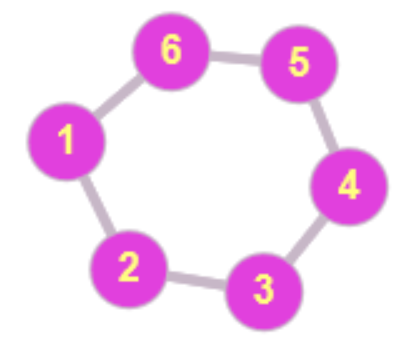 $\quad \mathbf{A} = \left({\begin{array}{rrrrrr}0&1&0&0&0&1\\1&0&1&0&0&0\\0&1&0&1&0&0\\0&0&1&0&1&0\\0&0&0&1&0&1\\1&0&0&0&1&0\\\end{array}}\right)
\quad \mathbf{L}_S = \left({\begin{array}{rrrrrr}2&-1&0&0&0&-1\\-1&2&-1&0&0&0\\0&-1&2&-1&0&0\\0&0&-1&2&-1&0\\0&0&0&-1&2&-1\\-1&0&0&0&-1&2\\\end{array}}\right)$
$\quad \mathbf{A} = \left({\begin{array}{rrrrrr}0&1&0&0&0&1\\1&0&1&0&0&0\\0&1&0&1&0&0\\0&0&1&0&1&0\\0&0&0&1&0&1\\1&0&0&0&1&0\\\end{array}}\right)
\quad \mathbf{L}_S = \left({\begin{array}{rrrrrr}2&-1&0&0&0&-1\\-1&2&-1&0&0&0\\0&-1&2&-1&0&0\\0&0&-1&2&-1&0\\0&0&0&-1&2&-1\\-1&0&0&0&-1&2\\\end{array}}\right)$
Fig. 1: The adjacency matrix $\mathbf{A}$ and the graph Laplacian $\Ll_S$ for a cyclic graph with six nodes.
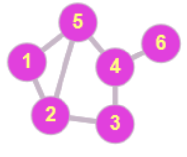 $\quad \mathbf{A} = \left({\begin{array}{rrrrrr}0&1&0&0&1&0\\1&0&1&0&1&0\\0&1&0&1&0&0\\0&0&1&0&1&1\\1&1&0&1&0&0\\0&0&0&1&0&0\\\end{array}}\right)
\quad \mathbf{L}_S = \left({\begin{array}{rrrrrr}2&-1&0&0&-1&0\\-1&3&-1&0&-1&0\\0&-1&2&-1&0&0\\0&0&-1&3&-1&-1\\-1&-1&0&-1&3&0\\0&0&0&-1&0&1\\\end{array}}\right)$
$\quad \mathbf{A} = \left({\begin{array}{rrrrrr}0&1&0&0&1&0\\1&0&1&0&1&0\\0&1&0&1&0&0\\0&0&1&0&1&1\\1&1&0&1&0&0\\0&0&0&1&0&0\\\end{array}}\right)
\quad \mathbf{L}_S = \left({\begin{array}{rrrrrr}2&-1&0&0&-1&0\\-1&3&-1&0&-1&0\\0&-1&2&-1&0&0\\0&0&-1&3&-1&-1\\-1&-1&0&-1&3&0\\0&0&0&-1&0&1\\\end{array}}\right)$
Fig. 2: The adjacency matrix $\mathbf{A}$ and the standard graph Laplacian $\Ll_S$ for a second graph with six nodes.
2. Graph signals and the Graph Fourier Transform
A signal $x$ on the graph $G$ is a function $x: V \rightarrow \mathbb{R}$ on the nodes of $G$. As the node set $V$ is ordered, we usually write every signal $x$ as a vector $x = (x(\node{v}_1), \ldots, x(\node{v}_n))^{\intercal}\in \mathbb{R}^n$. On the space $\mathcal{L}(G)$ of all signals, we have a natural inner product and norm given by $$y^\intercal x := \sum_{i=1}^n x(\node{v}_i) y(\node{v}_i), \quad \|x\|^2 := x^{\intercal} x = \sum_{i=1}^n x(\node{v}_i)^2. $$ The standard orthonormal basis in $\mathcal{L}(G)$ is given by the system $\{\delta_{\node{v}_1}, \ldots, \delta_{\node{v}_n}\}$ where the unit vectors $\delta_{\node{v}_j}$ satisfy $\delta_{\node{v}_j}(\node{v}_i) = \delta_{i,j}$.
The harmonic structure on the graph $G$ is determined by the graph Laplacian $\Ll$. As $\Ll$ is symmetric, this harmonic structure does not depend on the orientation of the edges in $G$. The graph Laplacian $\Ll$ allows to introduce a graph Fourier transform on $G$ in terms of its orthonormal eigendecomposition \begin{equation*} \mathbf{L}=\mathbf{U}\mathbf{M}_{\lambda} \mathbf{U^\intercal}. \end{equation*} Here, $\mathbf{M}_{\lambda} = \mathrm{diag}(\lambda) = \text{diag}(\lambda_1,\ldots,\lambda_{n})$ denotes the diagonal matrix with the increasingly ordered eigenvalues $\lambda_i$, $i \in \{1, \ldots, n\}$, of the graph Laplacian $\mathbf{L}$ as diagonal entries. The columns $u_1, \ldots, u_{n}$ of the orthonormal matrix $\mathbf{U}$ are normalized eigenvectors of $\mathbf{L}$ with respect to the eigenvalues $\lambda_1, \ldots, \lambda_n$. The ordered set $\hat{G} = \{u_1, \ldots, u_{n}\}$ of eigenvectors is an orthonormal basis for the space $\mathcal{L}(G)$. We call $\hat{G}$ the spectrum of the graph $G$.
In classical Fourier analysis, as for instance the Euclidean space or the torus, the Fourier transform can be defined in terms of the eigenvalues and eigenfunctions of the Laplace operator. In analogy, we consider the elements of $\hat{G}$, i.e., the eigenvectors $\{u_1, \ldots, u_{n}\},$ as the Fourier basis on the graph $G$. In particular, we can define the graph Fourier transform of $x$ as the vector \begin{equation*} \hat{x} := \mathbf{U^\intercal}x = (u_1^\intercal x, \ldots, u_n^\intercal x)^{\intercal}, \end{equation*} with the inverse graph Fourier transform given as \begin{equation*} x = \mathbf{U}\hat{x}. \end{equation*} The entries $\hat{x}_i = u_i^\intercal x$ of $\hat{x}$ are the frequency components or coefficients of the signal $x$ with respect to the basis functions $u_i$. For this reason, $\hat{x} : \hat{G} \to \Rr$ can be regarded as a function on the spectral domain $\hat{G}$ of the graph $G$. To keep the notation simple, we will however usually represent spectral distributions $\hat{x}$ as vectors $(\hat{x}_1, \ldots, \hat{x}_n)^{\intercal}$ in $\Rr^n$.
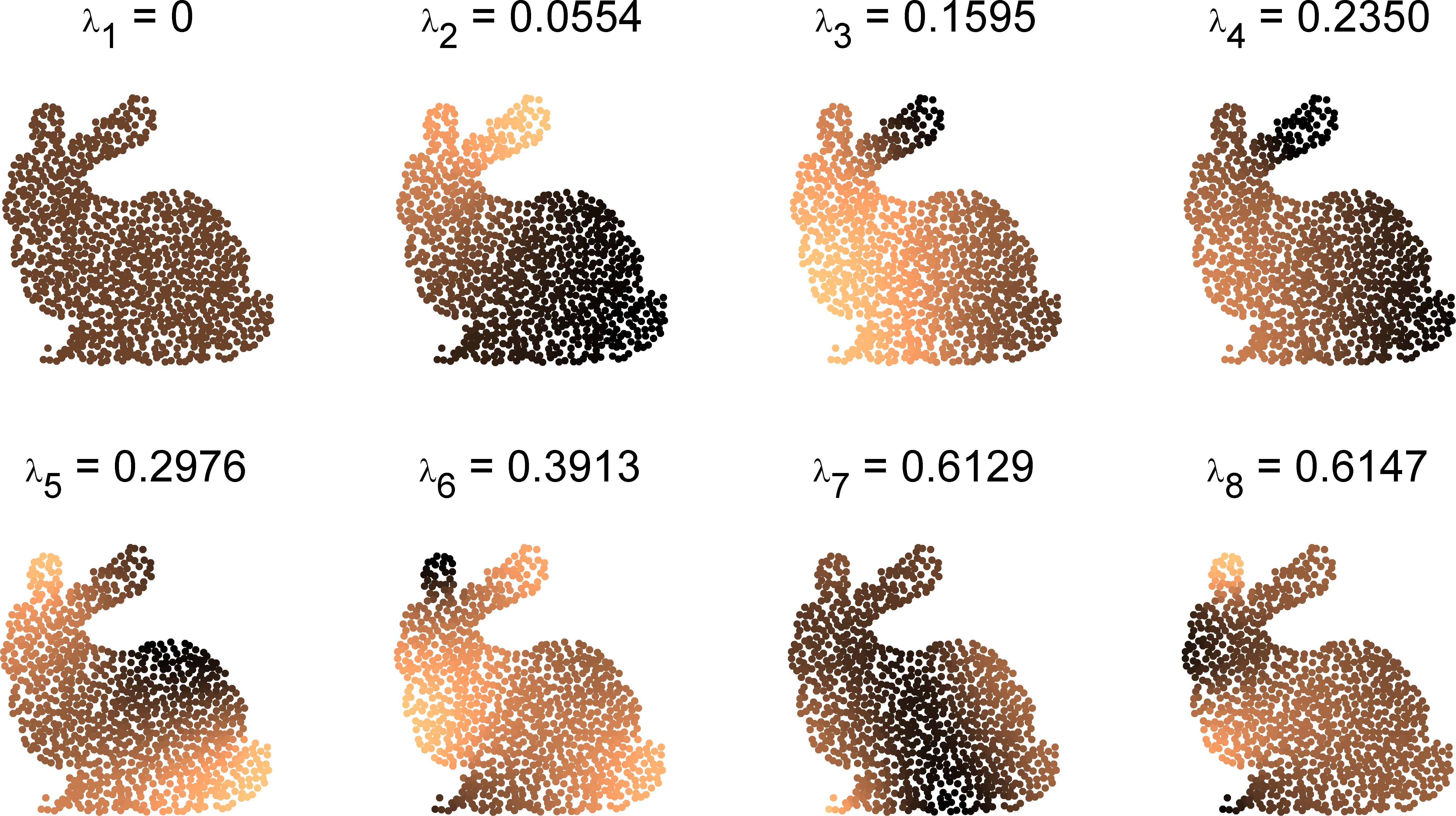
Fig. 3: The first 8 eigenvalues $\lambda_k$ and eigenfunctions $u_k$ of the Laplacian $\Ll_S$ on the bunny graph.
3. Convolution and Graph $C^{\ast}$-algebra
Based on the graph Fourier transform we can introduce a convolution operation between two graph signals $x$ and $y$. For this, we use an analogy to the convolution theorem in classical Fourier analysis linking convolution in the spatial domain to pointwise multiplication in the Fourier domain. In this way, the graph convolution for two signals $x,y \in \mathcal{L}(G)$ can be defined as \begin{equation*} x \ast y := \mathbf{U} \left ( \mathbf{M}_{\hat{x}} \hat{y} \right ) = \mathbf{U}\mathbf{M}_{\hat{x}}\mathbf{U^\intercal}y \label{eq:spectralfilter1}. \end{equation*} As before, $\mathbf{M}_{\hat{x}}$ denotes the diagonal matrix $\mathbf{M}_{\hat{x}} = \mathrm{diag}(\hat{x})$ and $\mathbf{M}_{\hat{x}} \hat{y} = (\hat{x}_1 \hat{y}_1, \ldots, \hat{x}_{n} \hat{y}_{n})$ gives the pointwise product of the two vectors $\hat{x}$ and $\hat{y}$. The convolution $\ast$ on $\mathcal{L}(G)$ has the following properties:
- $x \ast y = y \ast x$ (Commutativity),
- $(x \ast y) \ast z = x \ast (y \ast z)$ (Associativity),
- $(x + y) \ast z = x \ast z + (y \ast z)$ (Distributivity),
- $(\alpha x) \ast y = \alpha(y \ast x)$ for all $\alpha \in \Rr$ (Associativity for scalar multiplication).
4. Positive Definite Graph Basis Functions (GBF's)
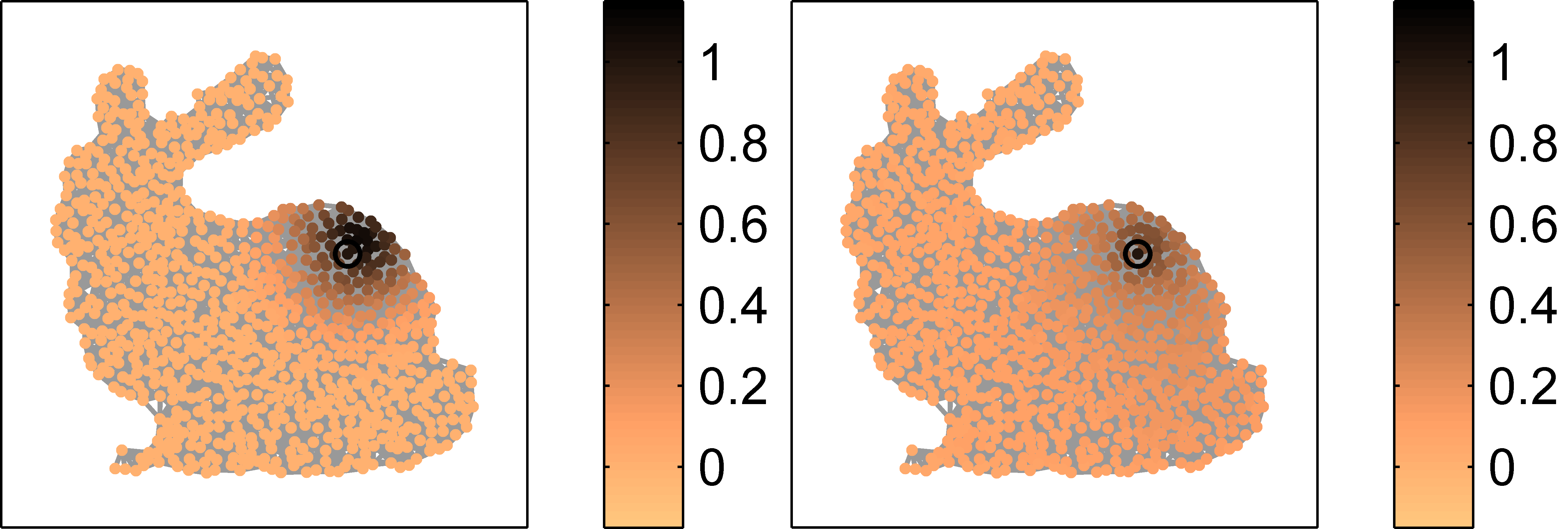
Fig. 4: Illustration of the normalized shifts $\mathbf{C}_{\delta_{\node{v}}} f$ of two GBF's. Left: $f = f_{e^{- 10 \mathbf{L}}}$. Right: $f = f_{\mathrm{pol},1}$. The ringed node corresponds to $\node{v}$.
Using the graph convolution, we can introduce a generalized translation of a signal $x$ on the graph $G$ by considering the signals \[ \mathbf{C}_{\delta_{\node{v}_k}} x = (x \ast \delta_{\node{v}_k}) = \mathbf{U} \mathbf{M}_{\hat{\delta}_{\node{v}_k}} \mathbf{U}^{\intercal} x. \] These signals can be interpreted as (generalized) translates of the basis function $x$ on the graph $G$. In fact, if $G$ has a group structure and the spectrum $\hat{G}$ consists of properly scaled characters of $G$, then the functions $\mathbf{C}_{\delta_{\node{v}_k}} x$ are shifts of the signal $x$ by the group element $\node{v}_k$. Although general graphs are not endowed with a group structure, this generalized notion of shift allows us to introduce positive definite functions on graphs.
Definition 1. A function $f: V \to \Rr$ on $G$ is called a positive definite (positive semi-definite) graph basis function (GBF) if the kernel matrix \[ \mathbf{K}_{f} = \begin{pmatrix} \mathbf{C}_{\delta_{\node{v}_1}} f(\node{v}_1) & \mathbf{C}_{\delta_{\node{v}_2}} f(\node{v}_1) & \ldots & \mathbf{C}_{\delta_{\node{v}_n}} f(\node{v}_1) \\ \mathbf{C}_{\delta_{\node{v}_1}} f(\node{v}_2) & \mathbf{C}_{\delta_{\node{v}_2}} f(\node{v}_2) & \ldots & \mathbf{C}_{\delta_{\node{v}_n}} f(\node{v}_2) \\ \vdots & \vdots & \ddots & \vdots \\ \mathbf{C}_{\delta_{\node{v}_1}} f(\node{v}_n) & \mathbf{C}_{\delta_{\node{v}_2}} f(\node{v}_n) & \ldots & \mathbf{C}_{\delta_{\node{v}_n}} f(\node{v}_n) \end{pmatrix}\] is symmetric and positive definite (positive semi-definite, respectively).
Positive definite GBF's can be characterized easily by a Bochner-type theorem in terms of their graph Fourier transform.
Theorem 2. A GBF $f$ is positive definite if and only if $\hat{f}_k > 0$ for all $k \in \{1, \ldots, n\}$. The Mercer decomposition of the corresponding kernel matrix $\mathbf{K}_f$ is given as \[ \mathbf{K}_f = \sum_{k=1}^n \hat{f}_k \, u_k \, u_k^{\intercal},\] i.e., the eigenvalues of $\mathbf{K}_f$ are precisely the Fourier coefficients $\hat{f}_k$ of $f$.
Important examples of GBF's
- For the diffusion GBF $f_{e^{-t \mathbf{L}}}$, the kernel matrix has the Mercer decomposition \[\mathbf{K}_{f_{e^{-t \mathbf{L}}}} = e^{ -t \mathbf{L}} = \sum_{k=1}^n e^{ -t \lambda_k} u_k u_k^{\intercal}.\]
- The variational spline GBF $f_{(\epsilon \mathbf{I}_n + \mathbf{L})^{-s}}$ is determined by the matrix \[\mathbf{K}_{f_{(\epsilon \mathbf{I}_n + \mathbf{L})^{-s}}} = (\epsilon \mathbf{I}_n + \mathbf{L})^{-s} = \sum_{k=1}^n \frac{1}{(\epsilon + \lambda_k)^s} u_k u_k^{\intercal}.\]
- The GBF $f_{\mathrm{pol},s}$ has a polynomial decay in the Fourier domain: \[\mathbf{K}_{f_{\mathrm{pol},s}} = \sum_{k=1}^n \frac{1}{k^s} u_k u_k^{\intercal}.\]
5. Interpolation with Graph Basis Functions
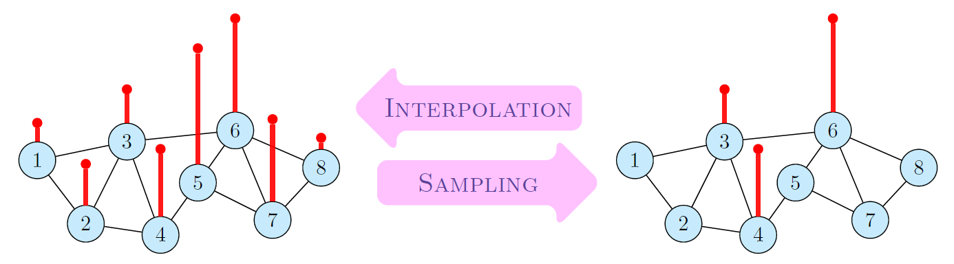
Fig. 5: Sampling and Interpolation of graph signals.
Positive definite GBF's can be applied in a simple and direct way to interpolate signal values $y(\node{w}_k)$ at a given node set $W = \{\node{w}_1, \ldots, \node{w}_N\}$. Thereby, the interpolation space \[\mathcal{N}_{K_f,W} = \left\{x \in \mathcal{L}(G) \ | \ x(\node{v}) = \sum_{k=1}^N c_k \mathbf{C}_{\delta_{\node{w}_k}} f(\node{v})\right\}. \] is spanned by the $N$ generalized shifts $\mathbf{C}_{\delta_{\node{w}_k}} f$ of the chosen GBF $f$. The positive definiteness of $f$ guarantees that we can find a unique interpolant $y^{\circ} \in \mathcal{N}_{K_f,W}$ such that \[ y^{\circ}(\node{w}) = y(\node{w}), \quad \text{for all} \; \node{w} \in W.\] The calculation of the interpolant is described in the following Algorithm 1.
Input: Signal values $y(\node{w}_1), \ldots, y(\node{w}_N)$ at the
node set $W = \{\node{w}_1, \ldots, \node{w}_N\}$.
A positive definite graph basis function $f$
Calculate the $N$ generalized translates $\mathbf{C}_{\delta_{\node{w}_1}} f = \delta_{\node{w}_1} \ast f, \ldots, \mathbf{C}_{\delta_{\node{w}_N}} f = \delta_{\node{w}_N} \ast f$.
Solve the linear system of equations \begin{equation*} \underbrace{\begin{pmatrix} \mathbf{C}_{\delta_{\node{w}_1}}f(\node{w}_1) & \mathbf{C}_{\delta_{\node{w}_2}}f(\node{w}_1) & \ldots & \mathbf{C}_{\delta_{\node{w}_N}}f(\node{w}_1) \\ \mathbf{C}_{\delta_{\node{w}_1}}f(\node{w}_2) & \mathbf{C}_{\delta_{\node{w}_2}}f(\node{w}_2) & \ldots & \mathbf{C}_{\delta_{\node{w}_N}}f(\node{w}_2) \\ \vdots & \vdots & \ddots & \vdots \\ \mathbf{C}_{\delta_{\node{w}_1}}f(\node{w}_N) & \mathbf{C}_{\delta_{\node{w}_2}}f(\node{w}_N) & \ldots & \mathbf{C}_{\delta_{\node{w}_N}}f(\node{w}_N) \end{pmatrix}}_{\mathbf{K}_{f,W}} \begin{pmatrix} c_1 \\ c_2 \\ \vdots \\ c_N \end{pmatrix} = \begin{pmatrix} y(\node{w}_1) \\ y(\node{w}_2) \\ \vdots \\ y(\node{w}_N) \end{pmatrix}. \end{equation*}
Calculate the GBF-interpolant \[ y^{\circ}(\node{v}) = \sum_{k=1}^N c_k \mathbf{C}_{\delta_{\node{w}_k}} f (\node{v}).\]
In the Matlab package GBFlearn the GBF-interpolant can be calculated via the command GBF_itpGBF. If the eigenvectors and eigenvalues of the graph Laplacian are given as G.U and G.Lambda, and the indices and values of the interpolation nodes are stored in idxW and yW, the GBF-interpolant can be calculated as follows:
%Calculate shifted basis functions for diffusion GBF
bf = GBF_genGBF(G.U,G.Lambda,idxW,'diffusion',10);

%Calculate GBF-interpolant
yInt = GBF_itpGBF(bf,idxW,yW);
An example of such an interpolation on the bunny graph is given in the following Fig. 6.
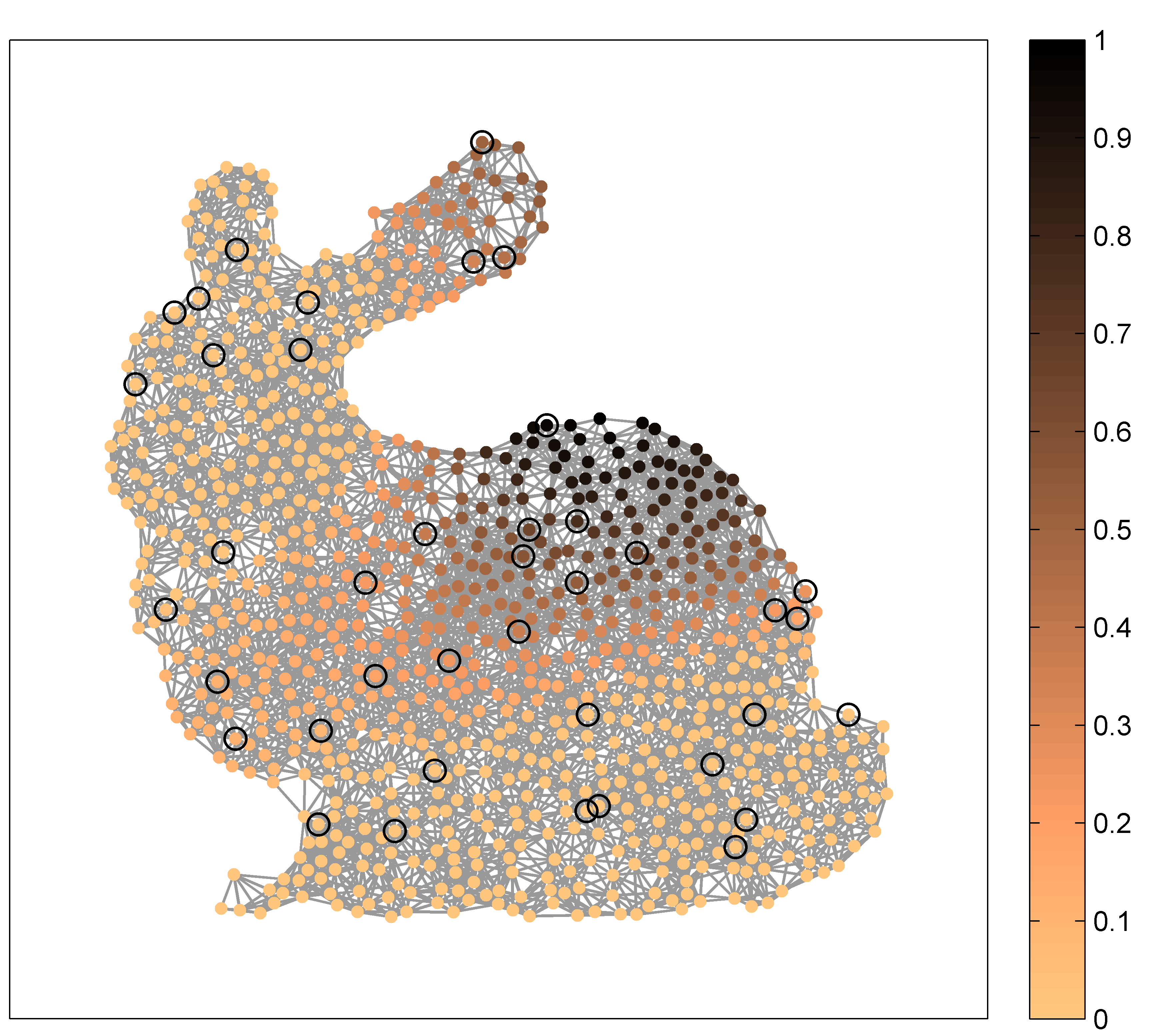
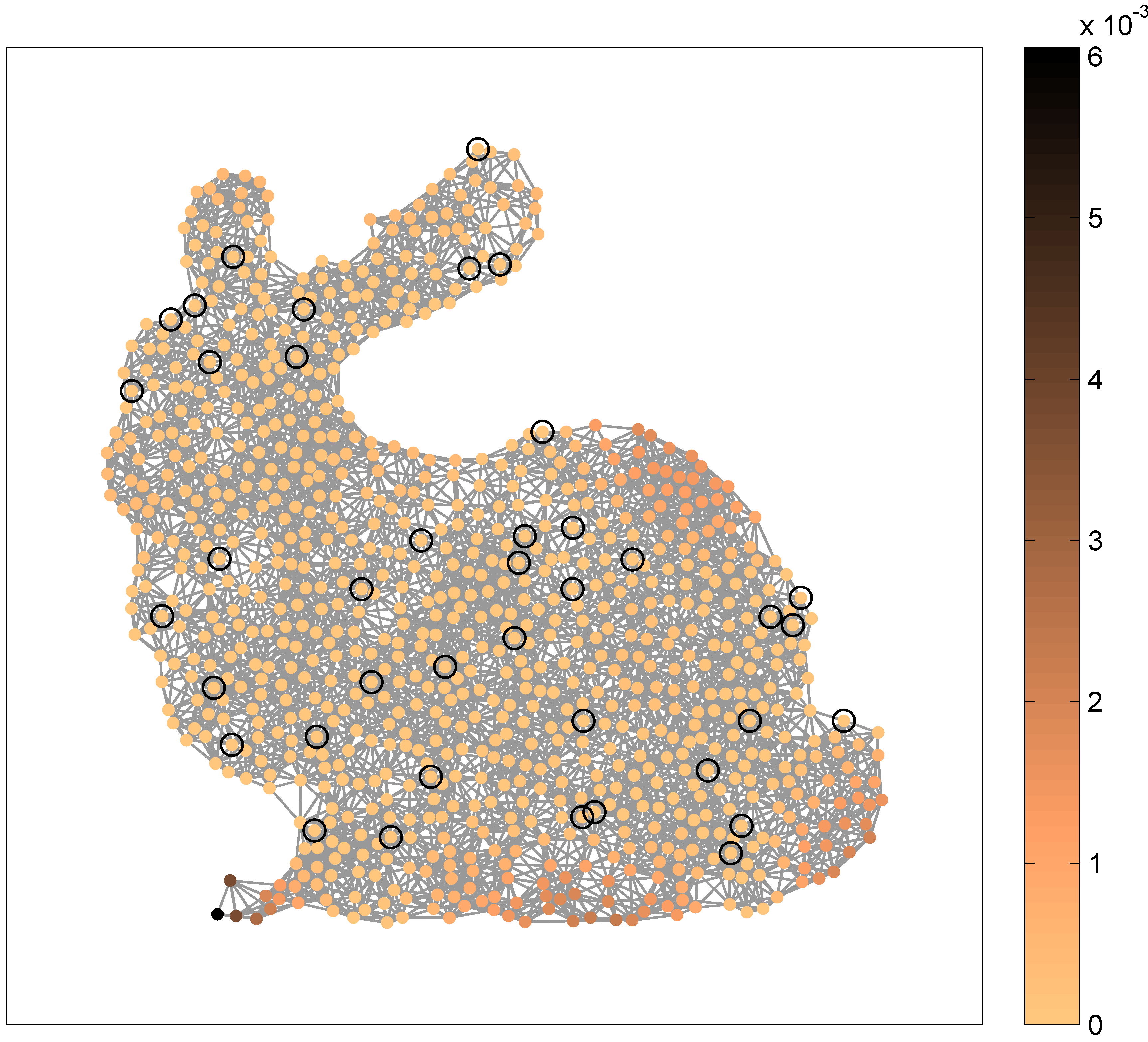
Fig. 6: GBF interpolation of the input signal $y = u_5$. Left: GBF interpolant $y^{\circ}$ for $N=40$ given nodes (out of $900$ nodes) and the GBF $f_{\mathrm{pol},4}$. Right: interpolation error $|y - y^{\circ}|$.
6. Classification with Graph Basis Functions
For kernel-based classification on graphs, GBF's offer a simple possibility to obtain predictors via the calculation of a regularized least squares (RLS) solution. For this, we calculate for given labels $y(\node{w}_1), \ldots, y(\node{w}_N) \in \{-1,1\}$ the minimizer $y^*$ of the RLS-functional \begin{equation*} \label{eq:RLSfunctionalpd} y^* = \underset{x \in \mathcal{N}_{K_f}}{\mathrm{argmin}} \left( \frac{1}{N} \sum_{i=1}^N |x(\node{w}_i)-y(\node{w}_i)|^2 + \gamma \, \hat{x}^\intercal \mathbf{M}_{1/\hat{f}} \hat{x} \right) \end{equation*} using a regularization parameter $\gamma>0$. Compared to the interpolant $y^{\circ}$ the RLS solution $y^* \in \mathcal{N}_{K_f}$ is smoother with respect to the norm $\|y\|_{K_f}^2 = \hat{y}^\intercal \mathbf{M}_{1/\hat{f}} \hat{y}$. Out of the RLS solution $y^*$, a binary classifier for the graph nodes can be calculated by taking $\mathrm{sign}(y^*)$. The single steps to calculate this predictor are summarized in the following Algorithm 2.
Input: Binary labels $y(\node{w}_1), \ldots, y(\node{w}_N) \in \{-1,1\}$ at the
node set $W = \{\node{w}_1, \ldots, \node{w}_N\}$,
A positive definite graph basis function $f$
Calculate the $N$ generalized translates $\mathbf{C}_{\delta_{\node{w}_1}} f = \delta_{\node{w}_1} \ast f, \ldots, \mathbf{C}_{\delta_{\node{w}_N}} f = \delta_{\node{w}_N} \ast f$.
Solve the linear system of equations (with regularization parameter $\gamma$) \begin{equation*} \underbrace{\begin{pmatrix} \mathbf{C}_{\delta_{\node{w}_1}}f(\node{w}_1) + \gamma N & \mathbf{C}_{\delta_{\node{w}_2}}f(\node{w}_1) & \ldots & \mathbf{C}_{\delta_{\node{w}_N}}f(\node{w}_1) \\ \mathbf{C}_{\delta_{\node{w}_1}}f(\node{w}_2) & \mathbf{C}_{\delta_{\node{w}_2}}f(\node{w}_2) + \gamma N & \ldots & \mathbf{C}_{\delta_{\node{w}_N}}f(\node{w}_2) \\ \vdots & \vdots & \ddots & \vdots \\ \mathbf{C}_{\delta_{\node{w}_1}}f(\node{w}_N) & \mathbf{C}_{\delta_{\node{w}_2}}f(\node{w}_N) & \ldots & \mathbf{C}_{\delta_{\node{w}_N}}f(\node{w}_N) + \gamma N \end{pmatrix}}_{\mathbf{K}_{f,W}+ \gamma N \mathbf{I}_N} \begin{pmatrix} c_1 \\ c_2 \\ \vdots \\ c_N \end{pmatrix} = \begin{pmatrix} y(\node{w}_1) \\ y(\node{w}_2) \\ \vdots \\ y(\node{w}_N) \end{pmatrix}. \end{equation*}
Calculate the regularized least squares solution $y^{*}$ and the binary predictor $\mathrm{sign} (y^{*})$ as \[ \mathrm{sign} (y^{*}(\node{v})) = \mathrm{sign} \left( \sum_{k=1}^N c_k \mathbf{C}_{\delta_{\node{w}_k}} f (\node{v}) \right).\]
In the Matlab package GBFlearn, binary GBF-classifiers can be computed with help of the command GBF_RLSGBF. Given the node indices idxW, the labels yW, and the regularization parameter gamma, the regularized least squares solution and the binary classification can be calculated as follows:
%Calculate shifted basis functions for diffusion GBF
bf = GBF_genGBF(G.U,G.Lambda,idxW,'diffusion',10);

%Calculate GBF-interpolant
yRLS = GBF_RLSGBF(bf,idxW,yW,gamma);

%Calculate binary GBF-classification
yClass = sign(yRLS);
As a final example, we use Algorithm 2 to classify the two moons in Fig. 7. To obtain the two supervised classifications in Fig. 7, we only needed 2 and 8 labeled nodes in this data set, respectively.

Fig. 7: Supervised binary classification of a two-moon data set (left) using a GBF regularized least squares method with 2 (middle) and 8 (right) labeled nodes (see implementation in GBFlearn).
GBF-classification on graphs can be improved by incorporating additional prior information in a semi-supervised setting. The details of this feature-augmentation procedure are described in [2]. Semi-supervised classification with feature-augmented GBF's is also implemented in GBFlearn.
Main publications
- [1] Erb, W. Graph Signal Interpolation with Positive Definite Graph Basis Functions. arXiv:1912.02069 (2019) (Preprint)
- [2] Erb, W. Semi-Supervised Learning on Graphs with Feature-Augmented Graph Basis Functions. arXiv:2003.07646 (2020) (Preprint)
Software
- GBFlearn: A software package for the interpolation, regression and classification of data on graphs.