A spherical Lissajous curve is defined in parametric form as \[\boldsymbol{\ell}^{(\boldsymbol{m})}_{\alpha}(t) = \Big( \sin(m_2 t) \cos (m_1 t - \alpha \pi), \ \sin(m_2 t) \sin (m_1 t - \textstyle\alpha \pi), \ \cos(m_2 t) \Big), \quad t \in \mathbb{R},\] with a frequency vector \(\boldsymbol{m} = (m_1, m_2) \in{\mathbb N}^{2}\) and a rotation parameter \(\alpha \in {\mathbb R}\). The curve \(\boldsymbol{\ell}^{(\boldsymbol{m})}_{\alpha}\) lies on the unit sphere \(\mathbb{S}^2= \{\boldsymbol{x} \in {\mathbb R}^3:\; x_1^2+x_2^2+x_3^2 = 1\}\) of the three-dimensional space \({\mathbb R}^3\) and describes a superposition of a latitudinal and a longitudinal harmonic motion determined by the frequencies \(m_1\) and \(m_2\). Two typical examples are illustrated in the Figure 1.
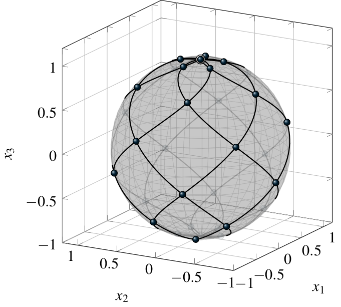
Fig. 1: Two spherical Lissajous curves \(\boldsymbol{\ell}^{(\boldsymbol{m})}_{0}\) with its intersection points. Left: \(\boldsymbol{\ell}^{(6,5)}_{0}\). Right: Animation of \(\boldsymbol{\ell}^{(7,6)}_{0}\).
In the following, we give a brief introduction to spherical Lissajous curves. In particular, we are interested in the number and type of the self-intersection points of these curves. The detailed proofs of the mathematical statements can be found in [1].
1. Intersection points of spherical Lissajous curves
If the frequencies \(m_1\) and \(m_2\) of \(\boldsymbol{\ell}^{(\boldsymbol{m})}_{\alpha}\) are relatively prime, Proposition 1 below implies that the time period to traverse the curve \(\boldsymbol{\ell}^{(\boldsymbol{m})}_{\alpha}\) once is \(2\pi\). In general, if \(g = \mathrm{gcd}(\boldsymbol{m})\) denotes the greatest common divisor of \(m_1\) and \(m_2\), then \(\boldsymbol{\ell}^{(\boldsymbol{m})}_{\alpha}\) can be rewritten as \(\boldsymbol{\ell}^{(\boldsymbol{m})}_{\alpha}(t) = \boldsymbol{\ell}^{(\boldsymbol{m}/g)}_{\alpha}( g t)\) and the period of \(\boldsymbol{\ell}^{(\boldsymbol{m})}_{\alpha}\) is \(2 \pi/g\). For the description of spherical Lissajous curves it is therefore enough to restrict ourselves to tuples \(\boldsymbol{m}\) of relatively prime numbers.
To extract the self-intersection points of the curve \(\boldsymbol{\ell}^{(\boldsymbol{m})}_{\alpha}\) we consider for \(t \in [0,2\pi)\) the sets \(\mathcal{A}^{(\boldsymbol{m})}(t) = \{ s \in [0,2\pi): \ \boldsymbol{\ell}^{(\boldsymbol{m})}_{\alpha}(s) = \boldsymbol{\ell}^{(\boldsymbol{m})}_{\alpha}(t) \}\) and the sampling points \[\begin{aligned} t^{(\boldsymbol{m})}_{l} &= \frac{l \pi}{m_1 m_2}, \quad l \in \{0,1, \ldots, 2m_1m_2-1\}, \label{eq-samples1}\\ t^{(\boldsymbol{m})}_{l+\frac12} &= \frac{(l + \frac12) \pi}{m_1 m_2}, \quad l \in \{0,1, \ldots, 2m_1m_2-1\}. \label{eq-samples2} \end{aligned}\]
Proposition 1 Let \(\mathrm{gcd}(\boldsymbol{m}) = 1\), i.e., the numbers \(m_1\) and \(m_2\) are relatively prime. If \(m_2\) is even, then \[\begin{array}{lll} (i) & \# \mathcal{A}^{(\boldsymbol{m})}(t) = m_2 & \text{if}\quad t \in \{\,t^{(\boldsymbol{m})}_{l}\,| \ l\in \{0,\ldots,2m_1m_2-1\}, \ l \equiv 0 \mod m_1 \},\\ (ii) & \# \mathcal{A}^{(\boldsymbol{m})}(t) = 2 & \text{if}\quad t \in \{\,t^{(\boldsymbol{m})}_{l}\,| \ l\in \{0,\ldots,2m_1m_2-1\}, \ l \not\equiv 0 \mod m_1 \}, \\ (iii) & \# \mathcal{A}^{(\boldsymbol{m})}(t) = 1 & \text{if}\quad t \in [0,2\pi) \setminus \{\,t^{(\boldsymbol{m})}_{l}\,|\, l\in \{0,\ldots,2m_1m_2-1\}\,\}. \end{array}\] If \(m_2\) is odd, then \[\begin{array}{lll} (i)' & \# \mathcal{A}^{(\boldsymbol{m})}(t) = m_2 & \text{if}\quad t \in \{\,t^{(\boldsymbol{m})}_{l}\,| \ l\in \{0,\ldots,2m_1m_2-1\}, \ l \equiv 0 \mod m_1 \}, \\ (ii)' & \# \mathcal{A}^{(\boldsymbol{m})}(t) = 2 & \text{if}\quad t \in \{\,t^{(\boldsymbol{m})}_{l+\frac12}\,| \ l\in \{0,\ldots,2m_1m_2-1\} \}, \\ (iii)' & \# \mathcal{A}^{(\boldsymbol{m})}(t) = 1 & \text{for all other $t \in [0,2\pi)$.} \end{array}\]
We can extract a series of properties from this result. If \(m_1\) and \(m_2\) are relatively prime we obtain as a consequence of Proposition 1 that the minimum period of \(\boldsymbol{\ell}^{(\boldsymbol{m})}_{\alpha}\) is \(2 \pi\). The points \(\boldsymbol{\ell}^{(\boldsymbol{m})}_{\alpha}(t)\) with \(\# \mathcal{A}^{(\boldsymbol{m})}(t) = m_2\) correspond to the north or the south pole of the sphere. Hence, in every period \([0,2\pi)\) the curve \(\boldsymbol{\ell}^{(\boldsymbol{m})}_{\alpha}\) traverses both poles \(m_2\) times. All other points \(\boldsymbol{\ell}^{(\boldsymbol{m})}_{\alpha}(t)\) with \(\# \mathcal{A}^{(\boldsymbol{m})}(t) = 2\) correspond to non-polar double points of the curve on the sphere, i.e., they are traversed twice by the curve as \(t\) varies from \(0\) to \(2 \pi\). Depending on whether \(m_2\) is even or odd, we get a different number of self-intersection points for \(\boldsymbol{\ell}^{(\boldsymbol{m})}_{\alpha}\). These numbers are summarized in Table 1.
| Curve \(\boldsymbol{\ell}^{(\boldsymbol{m})}_{\alpha}\) | Number of intersection points | Type of intersection points |
|---|---|---|
| \(m_2\) even | \(m_2 (m_1 -1) + 2\) | \(\begin{array}{l} \text{2 poles, traversed $m_2$ times in one period,} \\ \text{$m_2 (m_1 -1)$ non-polar double points} \end{array}\) |
| \(m_2\) odd | \(m_1 m_2 + 2\) | \(\begin{array}{l} \text{2 poles, traversed $m_2$ times in one period,} \\ \text{$m_1 m_2$ non-polar double points} \end{array}\) |
| \(m_2=1\) | \(m_1\) | \(\begin{array}{l} \text{$m_1$ non-polar double points} \end{array}\) |
Table 1: Number and type of intersection points for the curve
\(\boldsymbol{\ell}^{(\boldsymbol{m})}_{\alpha}\)
if \(m_1\), \(m_2\)
are relatively prime. For general \(\boldsymbol{m}\), the corresponding
numbers are obtained by considering the curve
\(\boldsymbol{\ell}^{(\boldsymbol{m}/g)}_{\alpha}\)
instead (\(g = \mathrm{gcd}(\boldsymbol{m})\)).
From the findings in Proposition 1 we see that an even frequency number \(m_2\) leads to a slightly different setup of intersection points than an odd \(m_2\). In the following, we will focus on the case that \(m_2\) is an even number. In this case the nodes \[\label{1709171731} \boldsymbol{\mathrm{LS}}^{(\boldsymbol{m})}_{\alpha} = \left\{\,\boldsymbol{\ell}^{(\boldsymbol{m})}_{\alpha}(t^{(\boldsymbol{m})}_{l})\,|\, l\in \{0,\ldots,2m_1m_2-1\} \,\right\}.\] contain the two poles of the sphere and give a simple characterization of all self-intersection points of the Lissajous curve \(\boldsymbol{\ell}^{(\boldsymbol{m})}_{\alpha}\).
Corollary 2 Let \(\mathrm{gcd}(\boldsymbol{m}) = 1\) and \(m_2\) even. Then, \(\boldsymbol{\mathrm{LS}}^{(\boldsymbol{m})}_\alpha\) is the set of all self-intersection points of the closed curve \(\boldsymbol{\ell}^{(\boldsymbol{m})}_{\alpha}(t)\), \(t \in [0,2\pi)\). \(\boldsymbol{\mathrm{LS}}^{(\boldsymbol{m})}_\alpha\) contains \(m_2 (m_1 -1) + 2\) points on the sphere \(\mathbb{S}^2\), including both poles that are traversed \(m_2\) times, and \(m_2(m_1-1)\) non-polar double points that are traversed \(2\) times by the curve \(\boldsymbol{\ell}^{(\boldsymbol{m})}_{\alpha}(t)\) as \(t\) varies from \(0\) to \(2\pi\).
2. The Lissajous intersection nodes as two interlacing spherical grids
In addition to the description given in Corollary 2, we can characterize the intersection points of the Lissajous curves also as the union of two interlacing rectangular grids in spherical coordinates. The construction for this second characterization can be performed for general frequencies \(\boldsymbol{m} = (m_1, m_2) \in{\mathbb N}^{2}\) where \(m_2\) is even. If \(m_1\) and \(m_2\) are not relatively prime the so obtained nodes can also be interpreted in terms of Lissajous curves. This relation will be discussed at the end of this section.
To describe the spherical Lissajous nodes we introduce the nodal index set \[\begin{equation}\label{eq:0911} \boldsymbol{\mathrm{I}}^{(\boldsymbol{m})}= \left\{ \,(i_1, i_2) \in {\mathbb N}_0^{2}\ \left|\begin {array}{ll} & 0\leq i_{1}\leq m_{1}, \; 0 \leq i_2 < 2 m_2, \\ & \text{$i_2 < m_2$, if $i_{1} \in \{0,m_1\}$}, \\ & \text{$i_{1} + i_{2}$ is even} \end{array}\right. \, \right\}. \end{equation}\] The set \(\boldsymbol{\mathrm{I}}^{(\boldsymbol{m})}\) is a disjoint union \(\boldsymbol{\mathrm{I}}^{(\boldsymbol{m})}= \boldsymbol{\mathrm{I}}^{(\boldsymbol{m})}_0 \cup \boldsymbol{\mathrm{I}}^{(\boldsymbol{m})}_1\) of the two sets \[\begin{equation} \label{eq:0901} \boldsymbol{\mathrm{I}}^{(\boldsymbol{m})}_0 = \{\boldsymbol{i} \in \boldsymbol{\mathrm{I}}^{(\boldsymbol{m})}\ | \ \text{$i_1$, $i_2$ are even} \, \}, \quad \boldsymbol{\mathrm{I}}^{(\boldsymbol{m})}_1 = \{\boldsymbol{i} \in \boldsymbol{\mathrm{I}}^{(\boldsymbol{m})}\ | \ \text{$i_1$, $i_2$ are odd} \, \}. \end{equation}\]
For \(\boldsymbol{i} = (i_1, i_2) \in \boldsymbol{\mathrm{I}}^{(\boldsymbol{m})}\) we obtain a relation to spherical coordinates by introducing the latitudinal and longitudinal angles \[\begin{equation*} \theta^{(m_1)}_{i_1} = \frac{i_1}{m_1} \pi \in [0,\pi], \qquad \varphi^{(m_2)}_{i_2} = \frac{i_2}{m_2} \pi \in [0,2\pi).\end{equation*}\] The set of nodes on the sphere \(\mathbb{S}^2\) corresponding to these spherical coordinates is given by \[\begin{equation} \label{eq:09172} \boldsymbol{\mathrm{LS}}^{(\boldsymbol{m})}= \left\{\, \boldsymbol{x}^{(\boldsymbol{m})}_{\boldsymbol{i}}\,\left|\,\boldsymbol{i}\in \boldsymbol{\mathrm{I}}^{(\boldsymbol{m})}\right.\right\}, \end{equation}\] with the points \(\boldsymbol{x}^{(\boldsymbol{m})}_{\boldsymbol{i}} \in \mathbb{S}^2\) defined by \[\begin{equation*}\boldsymbol{x}^{(\boldsymbol{m})}_{\boldsymbol{i}} = \left(\sin (\theta^{(m_1)}_{i_1}) \cos (\varphi^{(m_2)}_{i_2}), \sin (\theta^{(m_1)}_{i_1}) \sin (\varphi^{(m_2)}_{i_2}), \cos (\theta^{(m_1)}_{i_1})\right).\end{equation*}\] The cardinality of the set \(\boldsymbol{\mathrm{I}}^{(\boldsymbol{m})}\) can be determined from the simple structure of the sets \(\boldsymbol{\mathrm{I}}^{(\boldsymbol{m})}_0\) and \(\boldsymbol{\mathrm{I}}^{(\boldsymbol{m})}_1\). We have \[\begin{equation*} \#\boldsymbol{\mathrm{I}}^{(\boldsymbol{m})}_{0} = m_1 m_2 / 2, \quad \#\boldsymbol{\mathrm{I}}^{(\boldsymbol{m})}_{1} = m_1 m_2 / 2, \end{equation*}\] and thus \[\begin{equation*} \#\boldsymbol{\mathrm{I}}^{(\boldsymbol{m})} =\#\boldsymbol{\mathrm{I}}^{(\boldsymbol{m})}_{0} + \#\boldsymbol{\mathrm{I}}^{(\boldsymbol{m})}_{1} = m_1 m_2. \end{equation*}\] All points \(\boldsymbol{x}^{(\boldsymbol{m})}_{\boldsymbol{i}}\) with \(i_1 = 0\) describe the north pole of \(\mathbb{S}^2\) and all \(\boldsymbol{x}^{(\boldsymbol{m})}_{\boldsymbol{i}}\) with \(i_1 = m_1\) the south pole. Therefore, the cardinality of \(\boldsymbol{\mathrm{LS}}^{(\boldsymbol{m})}\) is smaller than \(\#\boldsymbol{\mathrm{I}}^{(\boldsymbol{m})}\). A simple counting gives \(\#\boldsymbol{\mathrm{LS}}^{(\boldsymbol{m})}= (m_1 -1) m_2 +2\). An example of a nodal index set \(\boldsymbol{\mathrm{I}}^{(\boldsymbol{m})}\) is illustrated in Figure 2.
The nodes \(\boldsymbol{\mathrm{LS}}^{(\boldsymbol{m})}\) can be characterized in terms of spherical Lissajous samples as follows.
Theorem 3 Let \(\boldsymbol{m} \in {\mathbb N}^2\) and \(m_2\) even. Then \[\begin{equation} \boldsymbol{\mathrm{LS}}^{(\boldsymbol{m})}= \bigcup_{\rho = 0}^{g-1} \left\{\,\boldsymbol{\ell}^{(\boldsymbol{m})}_{2 \rho/m_2} (t^{(\boldsymbol{m})}_{l})\ | \ l\in \{0,\ldots,2m_1m_2/g-1\} \,\right\},\end{equation}\] where \(t^{(\boldsymbol{m})}_{l}\) and \(\boldsymbol{\ell}^{(\boldsymbol{m})}_{\alpha}(t)\) denote the sampling points and the spherical Lissajous curves introduced above, and \(g = \mathrm{gcd}(\boldsymbol{m})\). In particular, if \(m_1\) and \(m_2\) are relatively prime, then \(\boldsymbol{\mathrm{LS}}^{(\boldsymbol{m})}\) corresponds to the self-intersection points \(\boldsymbol{\mathrm{LS}}^{(\boldsymbol{m})}_0\) of the curve \(\boldsymbol{\ell}^{(\boldsymbol{m})}_{0}\).
If \(m_1\) and the even \(m_2\) are relatively prime, Theorem 3 provides the second attempt to characterize the self-intersection points of the spherical Lissajous curves mentioned at the beginning of this section. If \(m_1\) and \(m_2\) are not relatively prime, it states that \(\boldsymbol{\mathrm{LS}}^{(\boldsymbol{m})}\) can be generated by time equidistant samples of at most \(g\) different Lissajous curves.
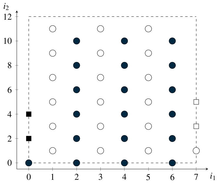
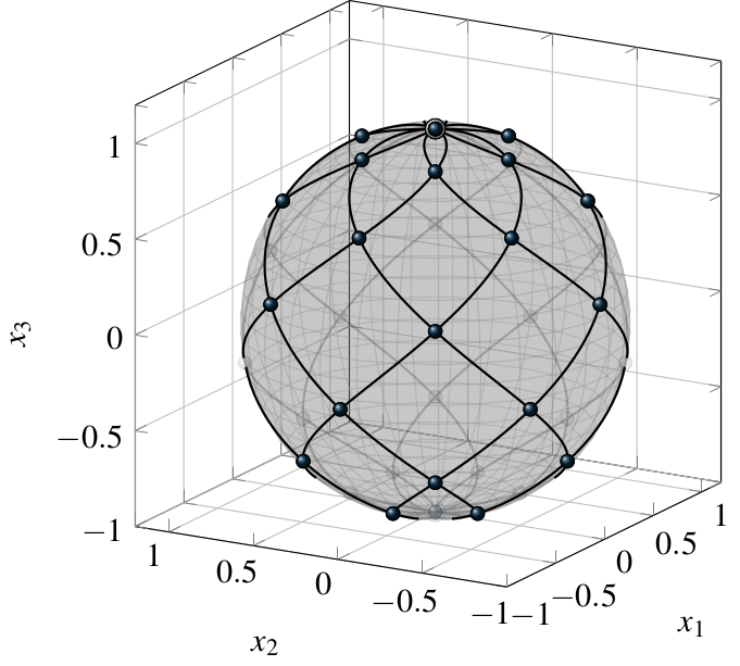
Fig. 2: The nodal index set \(\boldsymbol{\mathrm{I}}^{(7,6)}\) (left) and the corresponding spherical Lissajous nodes \(\boldsymbol{\mathrm{LS}}^{(7,6)}\) (right).
Main publication
- [1] Erb, W. A spectral interpolation scheme on the unit sphere based on the nodes of spherical Lissajous curves. IMA J. Numer. Anal. 40:2 (2020), 1330–1355 (Preprint) (Software LSphere)
Software
- LSphere: A software package that contains a Matlab implementation to plot spherical Lissajous curves and to compute spectral interpolants based on spherical Lissajous nodes.
Further literature on spherical Lissajous curves
A practical application of spherical Lissajous curves in MRI is described in- Ullisch, M. A navigator based rigid body motion correction for magnetic resonance imaging. Dissertation, Technische Hochschule Aachen (2012)
- Kaurov, V.
Lissajous Patterns on a Sphere Surface.
http://demonstrations.wolfram.com/LissajousPatternsOnASphereSurface/ (2011)